Example Codes: SAS #1 SAS #2 R #1
A descriptive statistic is a summary statistic that quantitatively describes or summarizes features from collected information. Some common types of descriptive statistics are measures of centrality such as arithmetic mean, median and mode, as well as measures of dispersion including standard deviation, range and interquartile range.
Measures of central tendency
Central tendency is a central or typical value for a probability distribution. Measures of central tendency are values that characterize the central location of a set of data. Some common measures of central tendency include arithmetic mean, median and mode.
Arithmetic mean
Arithmetic mean is the average value of data in a sample. The sample mean is calculated as the sum of all the numbers in the set of data divided by the number of observations:
![]()
Median
Median (![]() ) is the middle value of a sorted list of
numbers in a sample data. The value of median is not affected by the existence
of outliers in the sample data, that it is commonly used as an estimator of the
central value when outliers are detected.
) is the middle value of a sorted list of
numbers in a sample data. The value of median is not affected by the existence
of outliers in the sample data, that it is commonly used as an estimator of the
central value when outliers are detected.
Mode
Mode (![]() ) is the most frequent value that appears in
the sample data. A distribution can have
one unique mode (which is called a unimodal distribution), multiple modes or no
mode at all. Mode is a common measure of central tendency for categorical and
discrete data.
) is the most frequent value that appears in
the sample data. A distribution can have
one unique mode (which is called a unimodal distribution), multiple modes or no
mode at all. Mode is a common measure of central tendency for categorical and
discrete data.
Relationship between central tendency measures
For a symmetric and
unimodal distribution, the values of sample mean, median and mode coincide. If
the distribution is left-skewed, ![]() ; when the distribution is right-skewed,
; when the distribution is right-skewed, ![]() .
.
Example Code in SAS
data exam;
label score = 'Exam Score';
input score @@;
datalines;
81 97 78 99 77 81 84 86 86 97
85 86 94 76 75 42 91 90 88 86
97 97 89 69 72 82 83 81 80 81
;
PROC MEANS data = exam n mean median;
VAR score;
RUN;
PROC UNIVARIATE data = exam modes;
VAR score;
RUN;
Measures of spread
Measures of spread, also known as measures of dispersion, describe the variability in a set of data. In statistics, dispersion is the extent to which a distribution is stretched or squeezed. Common measures of spread are standard deviation, range and interquartile range.
Standard deviation
Standard deviation (SD) describes how far the data is spread out from the mean. SD is small when all the values in the data are close to the mean, whereas SD becomes larger if the dataset is more dispersed from the mean. The unbiased estimator of sample standard deviation is calculated as:
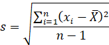
where ![]() are
observed values in the data,
are
observed values in the data, ![]() is
the sample mean,
is
the sample mean, ![]() is
the number of observations.
is
the number of observations.
Range
Range is the difference between the maximum and minimum values in a set of data. One advantage of range is that it can be easily calculated, however, its value is highly sensitive to outliers.
Interquartile range (IQR)
Interquartile range is calculated as the difference between the upper and the lower quartiles. The upper quartile refers to the 75th percentile of data values, while the lower quartile points to the 25th percentile of the data. Interquartile range reflects the variation of the middle 50% of observations in the set of data, and hence its value is not affected by extreme outliers.
Example Code in SAS
data exam;
label score = 'Exam Score';
input score @@;
datalines;
81 97 78 99 77 81 84 86 86 97
85 86 94 76 75 42 91 90 88 86
97 97 89 69 72 82 83 81 80 81
;
PROC MEANS data = exam std range qrange;
VAR score;
RUN;
Example Code in R
install.packages("DescTools")
# Load package DescTools for
function "Mode"
library(DescTools)
# input data
score <- c(81, 97, 78, 99, 71, 81, 84, 86, 86, 97, 85, 86, 94, 76, 75, 42, 91,
90, 88, 86, 97, 97, 89, 69, 72, 82, 83, 81, 80, 81)
# output mean, median and mode
mean(score)
median(score)
Mode(score)
# output standard deviation
sd(score)
# output range
diff(range(score))
# output inter-quartile range
IQR(score)